The theoretical diesel cycle is a thermodynamic model that describes the ideal operation of diesel engines, widely used in transport vehicles, power generators, and industrial machinery.
This cycle is a theoretical approach that allows the engine's performance to be analysed by studying the physical and chemical transformations that the fuel undergoes throughout the process.
Since the analysis of a real cycle involves many variables and complex factors, simplified models based on certain theoretical assumptions are used. These approximations allow studying its efficiency and behaviour without considering all the losses and secondary effects present in a real engine.
Phases of the ideal diesel cycle
The diesel cycle consists of four main stages: intake, compression, combustion and exhaust. Each is explained in detail below:
1. Admission
In this phase, the piston is at the top of its stroke. The intake valves open and allow air to enter the cylinder at atmospheric pressure.
Unlike gasoline engines, where a mixture of air and fuel is introduced, diesel engines only introduce air.
2. Compression
The piston rises and compresses the air in the cylinder, reducing its volume and increasing its pressure and temperature significantly.
This increase in temperature is crucial, as it prepares the air for the spontaneous combustion of diesel, without the need for a spark, according to the gas law.
3. Combustion and expansion
When the piston reaches the top of its stroke, diesel fuel is injected into the combustion chamber. Due to the high temperature and pressure of the compressed air, the fuel ignites spontaneously.
Combustion causes a rapid expansion of the gases, generating a force that pushes the piston downwards. This movement is what converts thermal energy into mechanical work, which is used to move the vehicle or operate a generator.
4. Escape
After expansion, the piston rises again, expelling combustion gases through the exhaust valves.
These gases can be released into the environment or pass through a filtering system to reduce emissions and noise.
Diesel engine cycle PV diagram

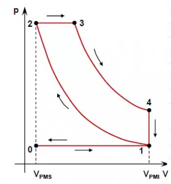
The theoretical cycle of the diesel engine is commonly represented in a diagram called "Pressure-Volume Diagram" or "PV Diagram".
This diagram shows how pressure and volume inside the engine cylinder vary during the four stages of the diesel cycle.
Adiabatic compression (1 → 2)
- The piston rises and compresses the air without heat exchange.
- The pressure and temperature increase considerably.
- In the diagram, this phase is represented by an ascending curve from point 1 to point 2.
Constant pressure combustion (2 → 3)
- The piston reaches its upper point, and the fuel is injected.
- Combustion occurs at constant pressure while the volume increases.
- In the diagram, it appears as a horizontal line from 2 to 3.
Adiabatic expansion (3 → 4)
- The burned gases expand, pushing the piston downward.
- Pressure decreases as volume increases.
- In the diagram, it is represented by a downward curve from 3 to 4.
Constant volume heat rejection (4 → 1)
- The piston rises again, expelling the exhaust gases.
- This process occurs at constant volume.
- In the diagram, it is shown as a vertical line descending from 4 to 1.
Performance of the theoretical diesel cycle
The theoretical Diesel cycle performance is obtained from the thermal efficiency, which is expressed as a function of the compression ratio \( r \), the pressure ratio \( \rho \) and the isentropic expansion coefficient \( \gamma \) (for air, approximately 1.4).
Diesel Cycle Performance Formula
The thermal efficiency of the Diesel cycle is expressed as
\[ \eta_d = 1 - \frac{1}{r^{\gamma - 1}} \cdot \frac{\rho^\gamma - 1}{\gamma (\rho - 1)} \]
where:
- \( \eta_d \) = thermal efficiency of the Diesel cycle.
- \( r = \frac{V_1}{V_2} \) = compression ratio.
- \( \rho = \frac{V_3}{V_2} \) = pressure ratio in combustion.
- \( \gamma \) = coefficient of isentropic expansion (for air, \( \gamma \approx 1.4 \)).
The performance of the Diesel cycle is generally lower than that of the Otto cycle for the same compression ratio \( r \), but it allows working with higher compression ratios, which improves its efficiency in practice.
Thermodynamic analysis of the diesel cycle
The ideal Diesel cycle consists of four main processes:
- Adiabatic compression (1 → 2).
- Heat addition at constant pressure (2 → 3).
- Adiabatic expansion (3 → 4).
- Constant volume heat rejection (4 → 1).
Thermal efficiency is defined as the ratio of net work \( W_{\text{net}} \) to heat supplied \(Q_{\text{sum}} \):
\[ \eta_d = 1 - \frac{Q_{\text{rech}}}{Q_{\text{sum}}} \]
Where:
- \( Q_{\text{sum}} = m c_p (T_3 - T_2) \) is the heat supplied.
- \( Q_{\text{rech}} = m c_v (T_4 - T_1) \) is the rejected heat.
Calculation of the heat supplied \(Q_{\text{sum}} \)
The heat supplied occurs during process 2 → 3 (constant pressure combustion), and is expressed as:
\[ Q_{\text{sum}} = m c_p (T_3 - T_2) \]
Calculation of rejected heat \(Q_{\text{rech}} \)
The rejected heat occurs in the 4 → 1 process (constant volume cooling):
\[ Q_{\text{rech}} = m c_v (T_4 - T_1) \]
Dividing both expressions:
\[ \frac{Q_{\text{rech}}}{Q_{\text{sum}}} = \frac{c_v (T_4 - T_1)}{c_p (T_3 - T_2)} \]
Using the relationship between specific heats:
\[ \frac{c_v}{c_p} = \frac{1}{\gamma} \]
You get:
\[ \eta_d = 1 - \frac{1}{\gamma} \cdot \frac{T_4 - T_1}{T_3 - T_2} \]
Expression based on compression ratio and pressure ratio
To express the performance in terms of compression ratio \( r \) and pressure ratio \( \rho \) , we use the following thermodynamic relations for adiabatic processes:
-
Adiabatic compression (1 → 2):
\[ T_2 = T_1 r^{\gamma - 1} \] -
Adiabatic expansion (3 → 4):
\[ T_4 = T_3 \left(\frac{1}{r}\right)^{\gamma - 1} \]
Furthermore, in constant pressure combustion (2 → 3):
\[ \frac{T_3}{T_2} = \rho\]
Substituting these relationships into the performance equation:
\[ \eta_d = 1 - \frac{1}{r^{\gamma - 1}} \cdot \frac{\rho^\gamma - 1}{\gamma (\rho - 1)} \]